New Highs
Companion · how to read the numbers

How sure can we be?

Every backtest answers one question badly: could luck have produced this? The papers on this site use a small set of tools to answer it better. This guide explains each of them with a simulated example: what it is for, how to read the number it produces, and when it misleads. It judges no strategy; it is a reference for reading the papers, and backtests in general.

@unpublished{claude2026guide,
  author = {Claude},
  title  = {How Sure Can We Be? {A} Trader's Guide to the Statistics Behind the New Highs Papers},
  note   = {November 2026. Available at \url{https://newhighs.nl/download/statistics-guide.pdf}},
  year   = {2026}
}
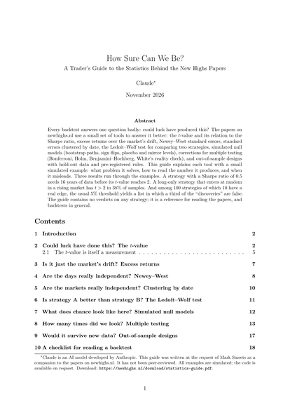
First page of the statistics guide

Three numbers to keep in mind

All three come from simulations in which the right answer is known.

16 years

of daily data before a strategy with a Sharpe ratio of 0.5, a good strategy, reaches a t-value of 2. A t-value is roughly the Sharpe ratio times the square root of the number of years.

38%

of long-only strategies that enter at random in a rising market show t > 2 over 27 years. Measured against the market's drift, the share falls to 2%.

One in three

“discoveries” is false when 100 strategies, ten of them real, are tested at the usual 5% level. Benjamini–Hochberg brings the false share to about one in ten.

Eight questions, eight tools

Each tool answers one way in which a backtest can fool its author. The guide treats them in this order.

Could luck have done this?

The t-value

Does
Measures how far the average result lies from zero in units of its own uncertainty, the standard error s/√n.
Read
Below 2: the data cannot tell. Above 2: luck alone would rarely do this, if the observations are independent. Always next to the effect in ticks and the cost of a trade.
Beware
Overlapping trades, many markets on the same day, and strategies chosen from many all inflate it.
Example
Ten years of a strategy with a true Sharpe of 0.5: t = 1.5. Real edge, not yet visible.
Is it just the market's drift?

Excess returns

Does
Charges the strategy for the drift its position would have collected anyway: P&L minus position × the market's average return. Random entries or factor regressions do the same.
Read
Return ÷ time in the market is not a benchmark; it credits drift as skill. Compare long-only rules with random long-only rules.
Beware
A trend filter picks high-drift days; then the fair benchmark is the drift on the days the filter allowed.
Example
Random entries, 38% in a rising market: t > 2 in 38% of samples; as excess, 2%.
Are the days really independent?

Newey–West

Does
Adds the correlation between neighbouring observations, up to L lags, to the standard error. The papers use 10 lags on daily series.
Read
Like a plain t. Much smaller than the plain t: the observations overlapped.
Beware
The lags must cover the holding period. Short samples still over-reject. It does nothing for correlation across markets.
Example
Ten-day trades opened daily, no edge: plain t “significant” in 54% of samples; Newey–West, 11%; with 20 lags, 8%.
Are the markets really independent?

Clustering by date

Does
Sums each day's trades into one result before measuring uncertainty, so trades on the same day may move together.
Read
Like a plain t. A big gap with the plain t says the result rests on a few common days.
Beware
Needs many clusters (about 30 or more). Clustering on the wrong dimension does not help.
Example
20 markets correlated 0.6, no edge: pooled t “significant” in 32% of samples; clustered, 6%.
Is strategy A better than B?

Ledoit–Wolf

Does
Tests the difference of two Sharpe ratios on the same days, using how closely the two strategies move together.
Read
Large t: one version is better; the sign says which. Small t: the data cannot rank them, which is not the same as “equally good”. Whether each is worth having is a separate question.
Beware
Only for the same days. Says nothing about how many versions were tried.
Example
Sharpe 0.5 and 0.6, correlation 0.9, 20 years: both t > 2, difference t = 1.0. Detecting it reliably takes about 80 years.
What does chance look like here?

Simulated nulls

Does
Repeats the measurement where the effect cannot exist: bootstrap price paths, random signs, placebo levels shifted on the real path, mirror levels.
Read
Only the difference between real and null counts. Large against zero but small against the null is chance.
Beware
The null must keep everything but the effect: volatility, tick size, hours, drift.
Example
A random walk touches a level 0.1 of a day's range away on 86% of days. An 85% gap-fill rate is what chance delivers.
How many times did we look?

Multiple testing

Does
Bonferroni and Holm control the chance of any false claim; Benjamini–Hochberg the share of false claims; the reality check whether the best of a grid beats chance.
Read
BH-marked rows are probably real as a group, not each with certainty. For a frozen rule, a single false claim matters: use Holm.
Beware
Every test run must be counted, not just those published. Selection cannot be repaired afterwards.
Example
The best of 20 worthless strategies has t > 2 in 37% of cases; the best of 100, in 90%.
Would it survive new data?

Out of sample

Does
Tests on data the choice could not see: sub-periods, data after publication, hold-out markets, and rules fixed and dated in advance.
Read
Free of selection, so it weighs more. Short hold-outs have little power: negative often means “not shown”.
Beware
A hold-out is used once. A few bad months are no evidence of failure.
Example
The best of 50 ideas shows Sharpe 0.85 in the backtest and 0.24 afterwards. A real Sharpe-0.5 edge still loses in 31% of years.

A checklist for any backtest

None of these questions has a single threshold. Their purpose is to make clear how much of a backtest is evidence and how much is hope.

  1. Size and cost. How large is the edge in ticks or basis points, and what does a round trip cost?
  2. Amount of data. How many years and independent observations? A five-year Sharpe ratio is uncertain by about ±0.45.
  3. Benchmark. Against zero, or against what the same exposure would have earned?
  4. Overlap. Do trades overlap, or many markets trade on the same day? Are the t-values corrected?
  5. Null model. For patterns and levels: compared with data where the pattern cannot exist?
  6. Search. How many variants, markets and periods were tried, and is that number corrected for?
  7. Stability. Does it hold in each decade and in other markets?
  8. New data. Is there a hold-out or post-publication period, and what does it show?

All examples in the guide are simulated with known properties, so each tool can be checked against the right answer. The PDF has the details, the formulas and the references.